Purpose of the exercise
To gain knowledge about the Ebsilon® Professional program environment and to develop a condensing steam power plant model allowing for calculations and determination of basic Rankine cycle parameters for defined input data.
Description of tasks to be performed
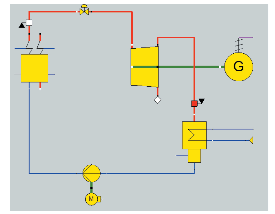
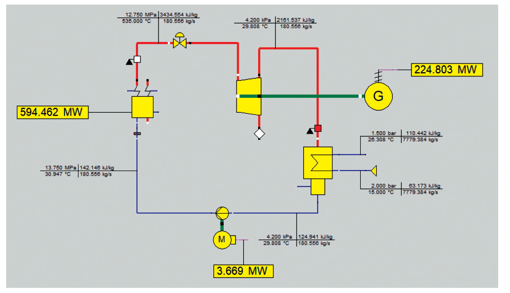
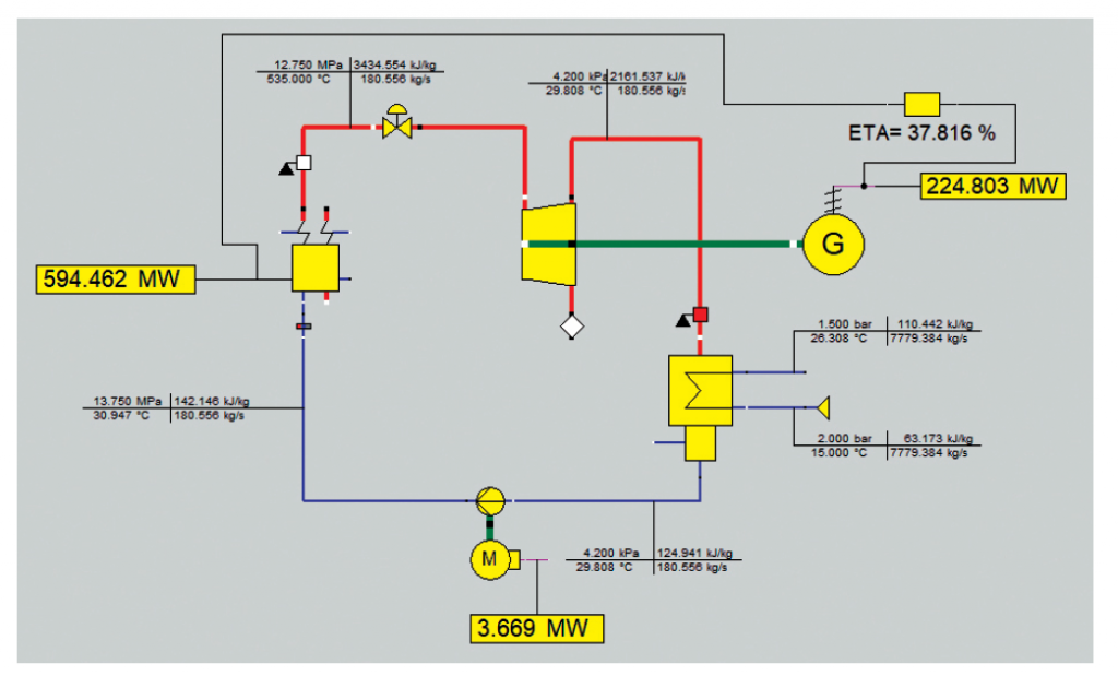
To perform the exercise, a model of a condensing steam power plant need to be prepared according to the diagram shown in Figure 1. The model should contain the following elements: boiler, control valve, steam turbine, condenser, pump and generator. The input data are shown in Table 1.
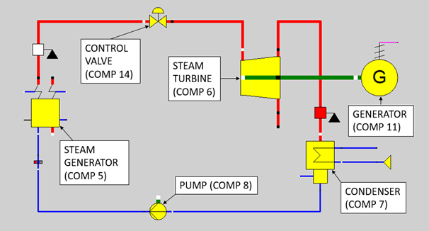
Table 1. Input data for the power plant model
| Parameter | Value | Unit | Component number |
|---|---|---|---|
| Live steam temperature | 535.00 | °C | 5 |
| Live steam pressure | 12.75 | MPa | 5 |
| Inlet pressure (nominal) | 12.40 | MPa | 6 |
| Mass flow start value | 650.00 | t/h | 46 |
| Condenser steam inlet pressure | 4.20 | kPa | 46 |
| Condenser Upper terminal temperature difference | 3.50 | K | 7 |
| Isentropic efficiency | 88.00 | % | 6 |
| Mechanical efficiency | 99.80 | % | 6 |
| Generator efficiency | 98.00 | % | 11 |
Uwaga: In the version Ebsilon® Professional 15 (or higher), to avoid the ‘Missing frequency’ error in the electric lines, change the Iteration report error option to ‘No’. To do so, go to option Extras → Model Options → Iteration → Select Nie (:0) for Report errors in the system of equations also for shafts and electric lines and click OK
Exercise modeling procedure
- . Open Ebsilon®Professional, save the file as Steam_Plant_model.ebs.
- Select and place the following components on the work area:
– Steam generator – Comp 5,
– Control valve – Comp 14,
– Steam turbine – Comp 6,
– Condenser – Comp 7,
– Pump – Comp 8,
– Motor – Comp 29,
– Generator – Comp 11. - Connect the selected components in the correct order as shown in the diagram in Figure 1.
- Supplement the model with elements allowing for entering input data:
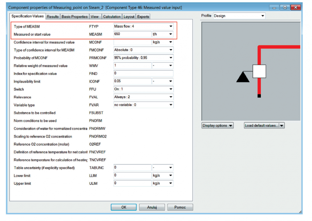
a) Place the Measuring point (Comp 46) component at the outlet steam line from the boiler. Inside the component, in the Type of MEASM (FTYP) field, select the Mass flow: 4 option, and then in the Measured or start value (MEASM) field, enter the value 650 t / h (Fig. 2).
b) Using the Measuring point (Comp 46) component, set the turbine outlet pressure at the Steam outlet line to 4.2 kPa.
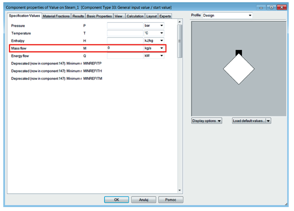
c) Additionally, on the Extraction 1 line from the steam turbine, place the component General input value / start value (Comp 33). Enter 0.0 kg / s in the Mass flow field (Fig. 3).
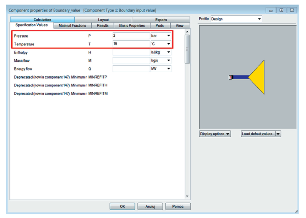
d) To input the cooling water parameters at the condenser inlet, select the component Boundary value (Comp 1) and connect it to the Cooling medium inlet line in the condenser component. Enter a value of 2.0 bar in the Pressure field and a value of 15.0 ° C in the Temperature field (Fig. 4).
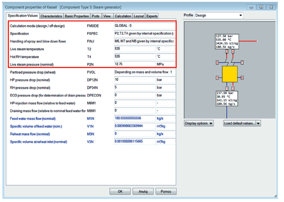
e) Complete the model with the values of temperature (Main steam temperature) and pressure (Main steam pressure) in the boiler component (Fig. 5), according to the data presented in table 1. Additionally, make sure that in the Specification and Handling of spray fields and blow down flows the options with index 0 are active.
- The remaining input data for the model should be defined using the components and methods presented in point 4, as summarized in Table 1. The last column of the table contains the names of components in which the indicated values should be entered. Figure 6 shows the model with the elements that allow for entering and changing the input data.
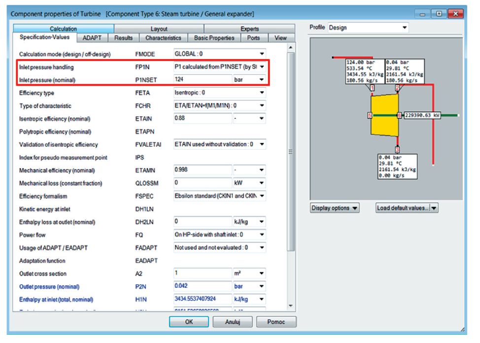
- In the turbine component, define the method of calculations – in the Inlet pressure handling field, select the option P1 calculated from P1NSET (by Stodola equation): 0 (Fig. 7). Additionally, in the field Inlet pressure (nominal), enter the value of the main steam pressure after the control valve to the turbine in accordance with Table 1.
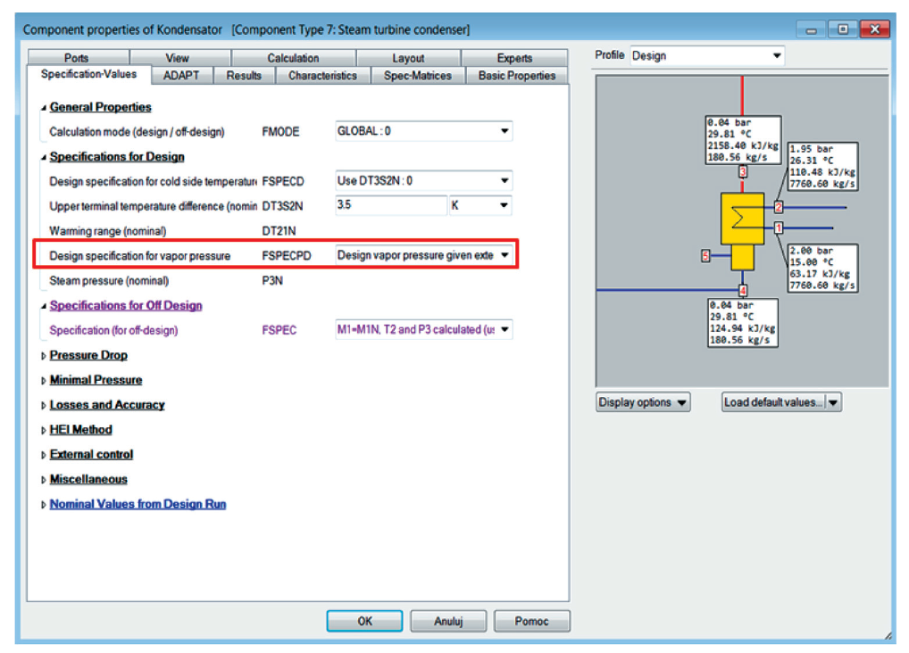
7. In the condenser component, in the Design specification for vapor pressure field, select Design vapor pressure given externally (in off design as start value): –1 as described in Figure 8.
8. Save the file with the developed model (Steam_Plant_model.ebs).
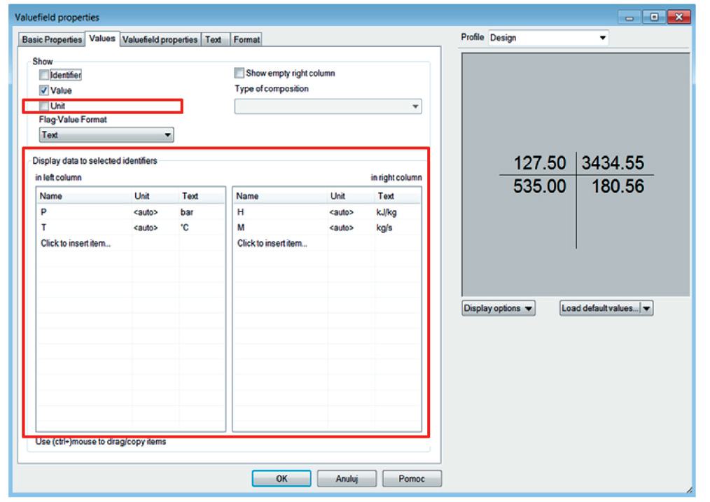
9. Supplement the model with elements enabling the visualization and presentation of selected parameters in characteristic points of the model circulation. To do this, select the Insert value-cross option from the toolbar and then indicate the line for which the parameter values will be displayed. By default, values for pressure, temperature, specific enthalpy and mass flow are displayed. The range of the presented parameters can be changed by double-clicking on the data table, then go to the Values tab. In the area marked in Figure 9, it is possible to add new or change the range of current parameters of a given line, which are presented in the model. Parameters can be selected from the list that expands after clicking in the Name column. Additionally, you can select the unit that should be displayed for a given parameter by expanding the list in the Unit column, and also activate the Unit option in the Show area. Using the Insert value-cross option, select the parameters of temperature, pressure, specific enthalpy and mass flow at characteristic points of the circulation, as shown in the diagram in Figure 9 (note: the values will only be displayed after the first calculations – see point 10). Display parameter values with the appropriate units (e.g. MPa, kJ / kg, ° C, kg / s).
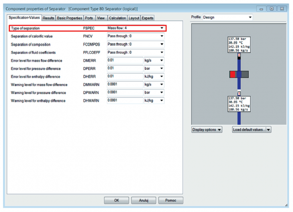
10. Perform calculations by running the simulation with the Simulation button or with the F9 key and verify the obtained results with the values presented in Figure 10. For the analyzed case, a message will appear informing about excess information about mass flow in the circulation – Overdetermination in 45 mass flow. In order to eliminate this error, an additional component, Separator (logical) – Comp 80, should be introduced into the model and placed on the feed water line before the boiler component (Fig. 10). Inside the separator component, select Mass flow: 4 in the Type of separation (FSPEC) field (Fig. 11). Details of errors in the model can be checked by selecting the Calculations tab on the toolbar, and then Error Analysis.
- Save the file with the model and calculation results (Steam_Plant_model.ebs).
- View the output at the generator terminals, the pump power, and the useful boiler heat output using the Insert Value-Cross option. NOTE: In order to enter an Insert Value-Cross marker on a given line, it must be extended. In the program, the power is marked with the letter Q. Additionally, in the Value field properties tab, select a yellow background – select the Fill option and then select a color. Compare your results with the results shown in Figure 10.
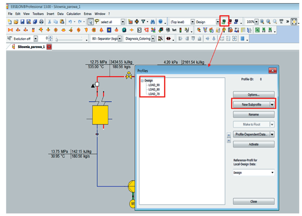
- Create new calculation profiles to simulate the operation of the condensing plant in the off-design mode, which represents the operation of the system under load conditions other than the rated load. To do this, on the toolbar, select the Edit profiles option, then New sub profile and after double-clicking on the newly created profile, change its name to LOAD_90 (Fig. 12). Repeat these steps and create two additional profiles LOAD_80 and LOAD_70. In off-design profiles, the amount of flowing steam should be defined at the level of 90% (LOAD_90), 80% (LOAD_80) and 70% (LOAD_70) of the nominal boiler capacity equal to 650 t / h. Enter the value of the fresh steam flow at component 46 on the fresh steam line from the boiler (see point 4a).
- Perform calculations for all defined calculation profiles (Design, LOAD_90, LOAD_80 and LOAD_70), and export the results for individual variants using the EBShtml function (File → Export → EBShtml).
- Save the final version of the file (Steam_Plant_results.ebs).
Additional task
- Calculate the energy efficiency of the cycle for all analyzed operating profiles of the condensing plant. To do this, use the Cycle efficiency meter (Comp 32) component, place it in the Design profile and configure it accordingly. Particular attention should be paid to the appropriate way of connecting the ports of this component – connect the Useful power port 1 with the electric power line from the generator, and the Expenditure port 2 (Sensible heat) with the logical line containing the useful power transmitted in the boiler. In the other off-design profiles, this component will be automatically entered. In component 32, select percent as the unit of efficiency. Compare the results with the results presented in Figure 13. Export the results using the EBShtml function.
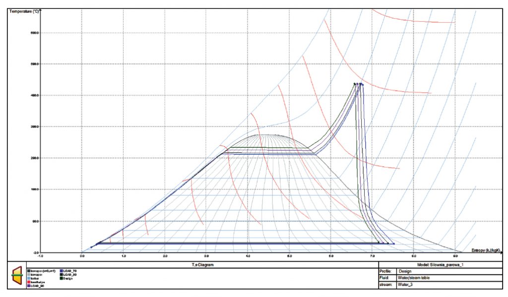
- Present the results on the temperature-entropy diagram (Fig. 14). To do this, select the Extras tab on the toolbar, then Diagrams, T-s Diagram and the Complete option. In the Profiles field, select all the created calculation profiles.
- Export the results using the EBShtml function. Save the file as Steam_Plant_additional_task.ebs.
Summary
The task was to familiarize the user with the Ebsilon® Professional program environment and to develop the first simulation model of a condensing steam power plant. The user knows how to identify components, connect them correctly, build the full structure of the simulation model and enter input data with a graphical presentation of selected calculation results.
Below are the solutions for the condensing steam power plant model presented in exercise 1, developed on the basis of the book:
Madejski P., Żymełka P., Wprowadzenie do komputerowych obliczeń i symulacji pracy systemów energetycznych w programie STEAG Ebsilon®Professional (Introduction to computations and simulations of energy systems operation using STEAG Ebsilon® Professional software]). Wydawnictwa AGH, Kraków 2020