Description of the simulation:
In our
example we recognize 9-pixel picture with the 9-neuron neural network. Black
pixel is represented by 1 and white is represented by -1.In this way we obtained test vectors that have 9 components. Using the Hebb
rule we have taught the network 3 shapes. Two of them remind a circle and a cross:
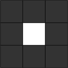
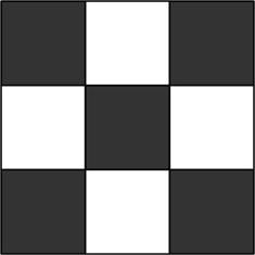
and the third one is clear picture which is
the vector that consists only -1.
X(1)=[1,1,1,1,-1,1,1,1,1]
X(2)=[1,-1,1,-1,1,-1,1,-1,1]
X(3)=[-1,-1,-1,-1,-1,-1,-1,-1,-1]
e.g. w12= w21= [1*1+1*(-1)+(-1)*(-1)]/9=1/9=0.111111
.
.
.
Complete matrix of weights is presented in
table:
|
|
Neuron 1 |
Neuron 2 |
Neuron 3 |
Neuron 4 |
Neuron 5 |
Neuron 6 |
Neuron 7 |
Neuron 8 |
Neuron 9 |
|
Neuron 1 |
0 |
0.111111 |
0.333333 |
0.111111 |
0.111111 |
0.111111 |
0.333333 |
0.111111 |
0.333333 |
|
Neuron 2 |
0.111111 |
0 |
0.111111 |
0.333333 |
-0.111111 |
0.333333 |
0.111111 |
0.333333 |
0.111111 |
|
Neuron 3 |
0.333333 |
0.111111 |
0 |
0.111111 |
0.111111 |
0.111111 |
0.333333 |
0.111111 |
0.333333 |
|
Neuron 4 |
0.111111 |
0.333333 |
0.111111 |
0 |
-0.111111 |
0.333333 |
0.111111 |
0.333333 |
0.111111 |
|
Neuron 5 |
0.111111 |
-0.111111 |
0.111111 |
-0.111111 |
0 |
-0.111111 |
0.111111 |
-0.111111 |
0.111111 |
|
Neuron 6 |
0.111111 |
0.333333 |
0.111111 |
0.333333 |
-0.111111 |
0 |
0.111111 |
0.333333 |
0.111111 |
|
Neuron 7 |
0.333333 |
0.111111 |
0.333333 |
0.111111 |
0.111111 |
0.111111 |
0 |
0.111111 |
0.333333 |
|
Neuron 8 |
0.111111 |
0.333333 |
0.111111 |
0.333333 |
-0.111111 |
0.333333 |
0.111111 |
0 |
0.111111 |
|
Neuron 9 |
0.333333 |
0.111111 |
0.333333 |
0.111111 |
0.111111 |
0.111111 |
0.333333 |
0.111111 |
0 |
The picture, which is presented in simulation mode, shows: input values of the
test vector (they are cleared after assigning to neurons outputs - before the second step), outputs
of weights adders, output values and output values from previous step (the
numbers in squares in column).
When the test vector,
which is passed to input of the network, is identical with one of the pattern vectors, the net
does not change its state. It recognizes also test vectors that are similar to patterns.
Sometimes we can see another feature of Hopfield network – remembering
relations between neighboring pixels without their values. As a result of
network activity we get the picture that is the reversed pattern.